Fitting Bayesian Distributed Lag Non-Linear Models with inlabru

Distributed lag non-linear models (DLNMs) are useful when an exposure can affect the response both non-linearly and with a delay. A common example is environmental epidemiology: today’s health outcome may depend on today’s temperature, yesterday’s temperature, and temperatures several days before, with a response curve that is not linear in temperature and not constant over lags.

The original DLNM formulation was described in Gasparrini et al.’s article, Distributed lag non-linear models, https://pmc.ncbi.nlm.nih.gov/articles/PMC2998707/. The standard R implementation is the dlnm package, described in the Journal of Statistical Software article Distributed Lag Linear and Non-Linear Models in R: The Package dlnm, https://www.jstatsoft.org/v43/i08/. Here I used dlnm::crossbasis() to build the cross-basis, then fitted the resulting Bayesian latent Gaussian model with inlabru.

The bdlnm package provides a convenient wrapper for fitting Bayesian DLNMs with R-INLA, as described here.

Instead of using a dedicated wrapper, some users may prefer to fit these models directly with inlabru. The goal here was to show how to turn a DLNM into:

• a matrix-based model component,
• a smooth Gaussian Markov random field prior on the tensor-product coefficients,
• an inlabru component fitted through generic3 and bm_matrix().

Model

Let \(Y_t\) be a count response and let \(x_t\) be an exposure observed over time. A DLNM with maximum lag \(L\) can be written as

\[Y_t \mid \mu_t \sim \operatorname{Poisson}(\mu_t), \qquad \log(\mu_t) = \alpha + \sum_{\ell = 0}^{L} f(x_{t-\ell}, \ell).\]

The surface \(f(x,\ell)\) is the object of interest. It encodes the exposure-response relationship along \(x\) and the delayed effect pattern along the lag dimension \(\ell\).

In the fitted example, I approximated this surface with a tensor-product basis:

\[f(x,\ell) = \sum_{j = 1}^{K_x} \sum_{k = 1}^{K_\ell} B_j^{(x)}(x) B_k^{(\ell)}(\ell) \theta_{jk}.\]

For each observation time \(t\), the corresponding row of the cross-basis matrix is

\[A_t = \sum_{\ell = 0}^{L} B^{(x)}(x_{t-\ell}) \otimes B^{(\ell)}(\ell),\]

so the distributed-lag contribution is simply \(A_t \theta\).

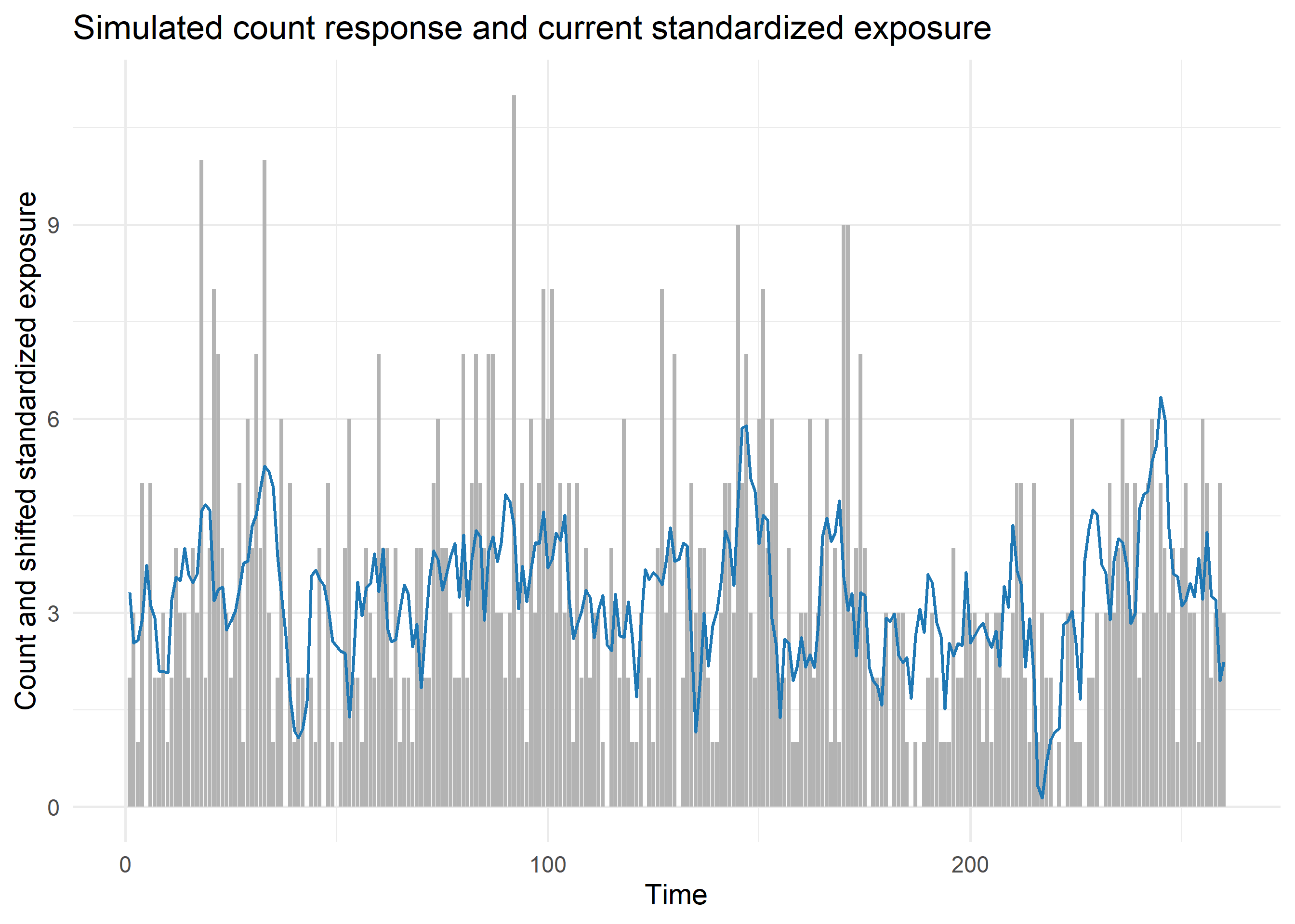
Simulated data

Let us now simulate some data so that the fitted surface could be compared with the truth. The exposure was autocorrelated, because lagged exposures are rarely independent in realistic time series. After simulation, I centred and scaled the exposure, so negative exposure values meant below-average exposure values rather than physically negative exposures. I set the baseline high enough for the latent-intensity comparison to be meaningful: with a much lower intercept, the response would have contained too many zeros to recover the latent intensity cleanly from one count series.

set.seed(7)

n <- 260L
max_lag <- 14L

x <- as.numeric(arima.sim(
  model = list(ar = 0.75),
  n = n + max_lag,
  sd = 0.6
))
x <- as.numeric(scale(x))

make_lagged_history <- function(x, max_lag) {
  idx <- seq_len(length(x) - max_lag) + max_lag
  out <- vapply(0:max_lag, function(lag) x[idx - lag], numeric(length(idx)))
  colnames(out) <- paste0("lag", 0:max_lag)
  out
}

x_history <- make_lagged_history(x, max_lag)
lag_grid <- 0:max_lag

true_lag_effect <- function(z, lag) {
  0.12 * z * exp(-lag / 5) -
    0.05 * pmax(z - 0.7, 0)^2 * exp(-lag / 10)
}

eta_dlnm <- rowSums(vapply(
  seq_along(lag_grid),
  function(j) true_lag_effect(x_history[, j], lag_grid[j]),
  numeric(nrow(x_history))
))

eta_intercept <- 1.2
eta <- eta_intercept + eta_dlnm
y <- rpois(nrow(x_history), lambda = exp(eta))

data.frame(
  time = seq_along(y),
  y = y,
  exposure = x[(max_lag + 1):length(x)]
) |>
  ggplot(aes(x = time)) +
  geom_col(aes(y = y), fill = "grey70", width = 0.9) +
  geom_line(aes(y = exposure + mean(y)), colour = "#1f78b4", linewidth = 0.6) +
  labs(
    x = "Time",
    y = "Count and shifted standardized exposure",
    title = "Simulated count response and current standardized exposure"
  )

Cross-basis

I built the cross-basis from a spline basis along the exposure axis and a spline basis along the lag axis. To do so, I used dlnm::crossbasis() directly, with one row per observed exposure history. The example used ten basis functions in each direction, so the tensor basis was fairly flexible while the smoothing prior still controlled roughness. Its columns were ordered in exposure-basis blocks, with the lag-basis index varying fastest:

\[\theta = (\theta_{11}, \ldots, \theta_{1K_\ell}, \theta_{21}, \ldots, \theta_{2K_\ell}, \ldots, \theta_{K_xK_\ell})^\top.\]

df_exposure <- 10L
df_lag <- 10L

cross_basis <- crossbasis(
  x_history,
  lag = c(0, max_lag),
  argvar = list(
    fun = "bs",
    df = df_exposure,
    degree = 3,
    intercept = FALSE
  ),
  arglag = list(
    fun = "bs",
    df = df_lag,
    degree = 3,
    intercept = TRUE
  )
)

k_exposure <- attr(cross_basis, "df")[1]
k_lag <- attr(cross_basis, "df")[2]

A_cross_dense <- scale(unclass(cross_basis), center = TRUE, scale = FALSE)
A_cross <- Matrix(A_cross_dense, sparse = TRUE)

dim(A_cross)

[1] 260 100

summary(cross_basis)

CROSSBASIS FUNCTIONS
observations: 260 
range: -3.119498 to 3.076913 
lag period: 0 14 
total df:  100 

BASIS FOR VAR:
fun: bs 
knots: -1.093494 -0.6584627 -0.3542118 -0.01597439 0.2933175 0.5745101 1.082654 ... 
degree: 3 
intercept: FALSE 
Boundary.knots: -3.119498 3.076913 

BASIS FOR LAG:
fun: bs 
knots: 2 4 6 8 10 12 
degree: 3 
intercept: TRUE 
Boundary.knots: 0 14 

Column centering separated the intercept from the cross-basis contribution. Without it, the intercept and parts of the spline surface could compete for the same constant shift.

Tensor-product prior

The 10 by 10 cross-basis introduced 100 latent coefficients. Without a structured prior, those coefficients could vary almost independently, which would make the surface too sensitive to Poisson noise and to sparsely observed exposure-lag combinations. The regularisation therefore had to work in both directions of the tensor product: neighbouring exposure-basis coefficients should be similar for a fixed lag pattern, and neighbouring lag-basis coefficients should be similar for a fixed exposure-response pattern.

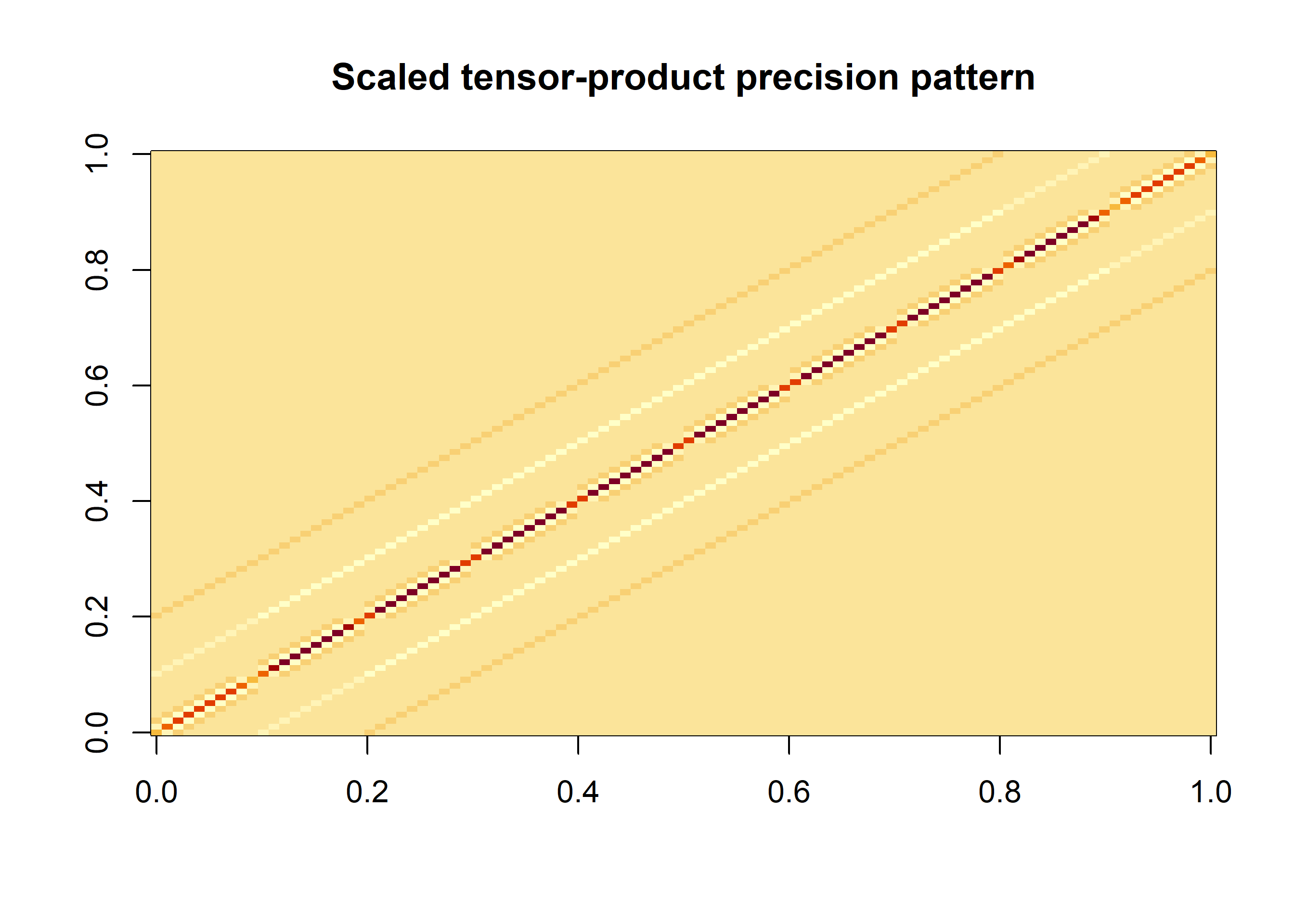
A convenient way to encode this was a Kronecker-sum precision matrix with separate smoothing strengths:

\[Q = \tau_\ell \left(Q_\ell \otimes I_x\right) + \tau_x \left(I_\ell \otimes Q_x\right),\]

where \(Q_x\) and \(Q_\ell\) are second-order random-walk precision matrices along the exposure and lag bases. The first term penalised roughness along the lag direction within each exposure-basis block. The second term penalised roughness along the exposure direction within each lag-basis block. The two precision parameters allowed the fitted surface to be smoother in one direction than in the other, which was useful because exposure-response curvature and lag decay need not have the same scale.

rw_precision <- function(k, order = 2) {
  D <- diff(Diagonal(k), differences = order)
  crossprod(D)
}

scale_rw2_precision <- function(Q) {
  k <- nrow(Q)
  constraints <- list(
    A = rbind(rep(1, k), seq_len(k)),
    e = c(0, 0)
  )
  INLA::inla.scale.model(Q, constr = constraints)
}

rw_order_exposure <- 2L
rw_order_lag <- 2L

Q_exposure <- scale_rw2_precision(
  rw_precision(k_exposure, order = rw_order_exposure)
)
Q_lag <- scale_rw2_precision(
  rw_precision(k_lag, order = rw_order_lag)
)

R_lag <- kronecker(Diagonal(k_exposure), Q_lag)
R_exposure <- kronecker(Q_exposure, Diagonal(k_lag))

Q_cross_display <- R_lag + R_exposure

rankdef_cross <- rw_order_exposure * rw_order_lag

image(as.matrix(Q_cross_display), main = "Scaled tensor-product precision pattern")

The marginal RW2 precision matrices were scaled with INLA::inla.scale.model() before the tensor-product terms were formed. This made the two precision hyperparameters more directly comparable. The tensor-product precision was intrinsic: since each RW2 precision has a two-dimensional null space, the Kronecker-sum precision had rank deficiency \(2 \times 2 = 4\). This rank deficiency was passed to generic3 through rankdef.

Fit with inlabru

The important inlabru detail is the mapper. The component received A_cross, a sparse matrix with one row per observation and one column per latent coefficient. The mapper bm_matrix(ncol(A_cross)) told inlabru that this component should be evaluated by matrix multiplication.

pc_prec <- list(
  prior = "pc.prec",
  param = c(1, 0.01)
)

components <- ~
  Intercept(
    1,
    mean.linear = 0,
    prec.linear = 0.01
  ) +
  dlnm(
    A_cross,
    model = "generic3",
    mapper = bm_matrix(ncol(A_cross)),
    Cmatrix = list(R_lag, R_exposure),
    rankdef = rankdef_cross,
    constr = TRUE,
    hyper = list(
      prec1 = pc_prec,
      prec2 = pc_prec
    )
  )

likelihood <- bru_obs(
  y ~ Intercept + dlnm,
  family = "poisson",
  data = data.frame(y = y)
)

fit_dlnm <- bru(
  components,
  likelihood,
  options = list(
    verbose = FALSE,
    bru_verbose = 0
  )
)

fit_dlnm$summary.fixed

              mean         sd 0.025quant 0.5quant 0.975quant     mode
Intercept 1.128264 0.03615628   1.057335 1.128274   1.199133 1.128274
                   kld
Intercept 7.617842e-11

fit_dlnm$summary.hyperpar

                                        mean        sd 0.025quant 0.5quant
Precision for Cmatrix[[1]] for dlnm 449.5433 1059.8757   12.76912 176.0293
Precision for Cmatrix[[2]] for dlnm 445.2669  752.3627   22.60053 226.1602
                                    0.975quant     mode
Precision for Cmatrix[[1]] for dlnm   2613.487 29.76736
Precision for Cmatrix[[2]] for dlnm   2236.180 57.65692

Linear predictor and latent intensity

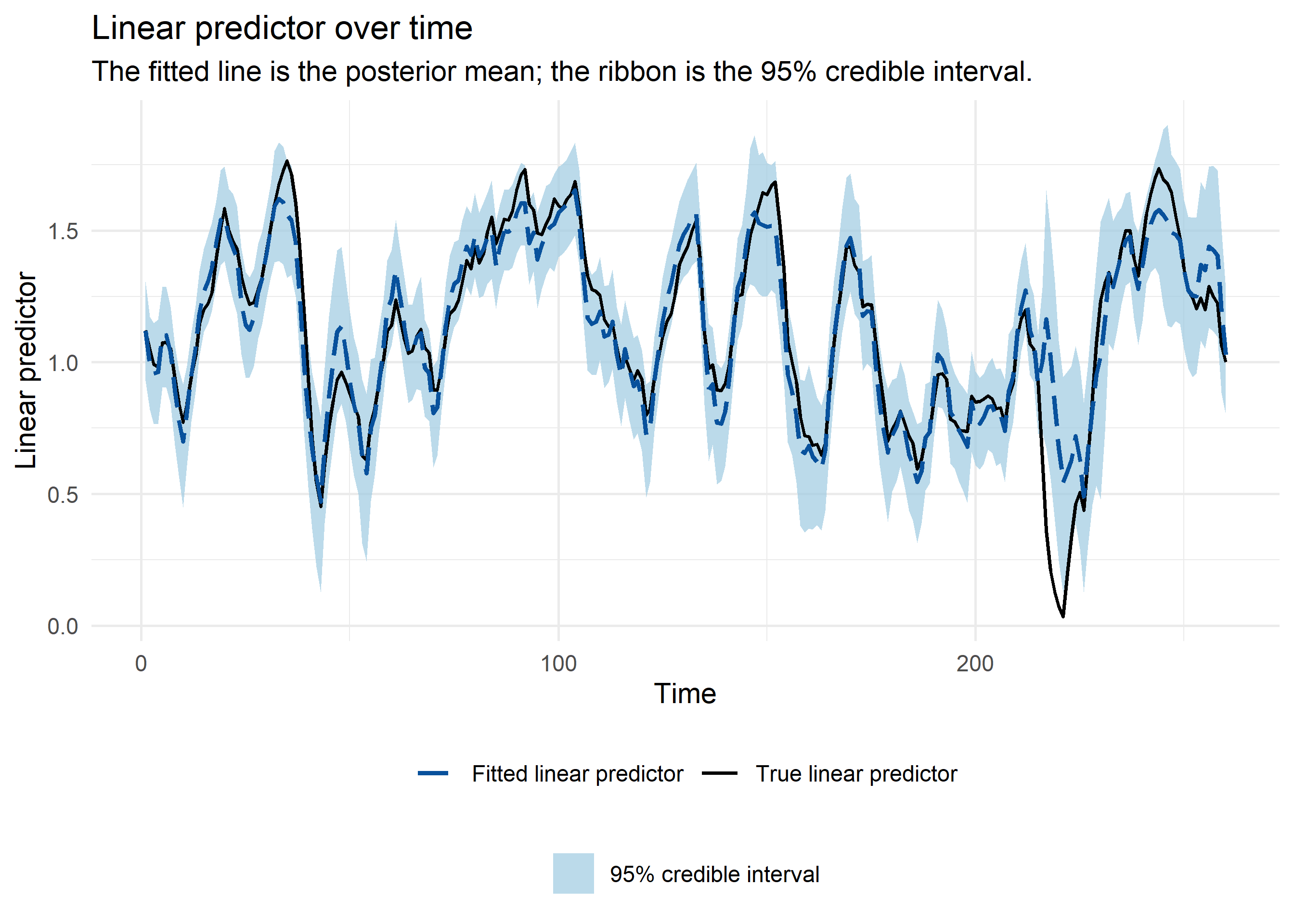
Because the data were simulated, the true linear predictor \(\eta_t = \alpha + \eta_{\mathrm{DLNM},t}\) and the true latent intensity \(\lambda_t = \exp(\eta_t)\) were known. This made it possible to compare the fitted linear predictor and fitted intensity directly with their simulated counterparts over time.

eta_prediction <- predict(
  fit_dlnm,
  formula = ~ data.frame(eta = Intercept + dlnm),
  n.samples = 1000,
  seed = 20260426
)

mu_prediction <- predict(
  fit_dlnm,
  formula = ~ data.frame(mu = exp(Intercept + dlnm)),
  n.samples = 1000,
  seed = 20260426
)

prediction_df <- data.frame(
  time = seq_along(y),
  eta_true = eta,
  eta_mean = eta_prediction$mean,
  eta_q025 = eta_prediction$q0.025,
  eta_q975 = eta_prediction$q0.975,
  mu_true = exp(eta),
  mu_mean = mu_prediction$mean,
  mu_q025 = mu_prediction$q0.025,
  mu_q975 = mu_prediction$q0.975
)

ggplot(prediction_df, aes(x = time)) +
  geom_ribbon(
    aes(
      ymin = eta_q025,
      ymax = eta_q975,
      fill = "95% credible interval"
    ),
    alpha = 0.7
  ) +
  geom_line(
    aes(
      y = eta_true,
      colour = "True linear predictor",
      linetype = "True linear predictor"
    ),
    linewidth = 0.7
  ) +
  geom_line(
    aes(
      y = eta_mean,
      colour = "Fitted linear predictor",
      linetype = "Fitted linear predictor"
    ),
    linewidth = 0.85
  ) +
  scale_colour_manual(
    values = c(
      "True linear predictor" = "black",
      "Fitted linear predictor" = "#08519c"
    )
  ) +
  scale_linetype_manual(
    values = c(
      "True linear predictor" = "solid",
      "Fitted linear predictor" = "longdash"
    )
  ) +
  scale_fill_manual(
    values = c("95% credible interval" = "#9ecae1")
  ) +
  guides(
    fill = guide_legend(order = 2),
    colour = guide_legend(order = 1),
    linetype = guide_legend(order = 1)
  ) +
  labs(
    x = "Time",
    y = "Linear predictor",
    colour = NULL,
    linetype = NULL,
    fill = NULL,
    title = "Linear predictor over time",
    subtitle = "The fitted line is the posterior mean; the ribbon is the 95% credible interval."
  ) +
  theme(
    legend.position = "bottom",
    legend.box = "vertical"
  )

ggplot(prediction_df, aes(x = time)) +
  geom_ribbon(
    aes(
      ymin = mu_q025,
      ymax = mu_q975,
      fill = "95% credible interval"
    ),
    alpha = 0.7
  ) +
  geom_line(
    aes(
      y = mu_true,
      colour = "True latent intensity",
      linetype = "True latent intensity"
    ),
    linewidth = 0.7
  ) +
  geom_line(
    aes(
      y = mu_mean,
      colour = "Fitted latent intensity",
      linetype = "Fitted latent intensity"
    ),
    linewidth = 0.85
  ) +
  scale_colour_manual(
    values = c(
      "True latent intensity" = "black",
      "Fitted latent intensity" = "#08519c"
    )
  ) +
  scale_linetype_manual(
    values = c(
      "True latent intensity" = "solid",
      "Fitted latent intensity" = "longdash"
    )
  ) +
  scale_fill_manual(
    values = c("95% credible interval" = "#9ecae1")
  ) +
  guides(
    fill = guide_legend(order = 2),
    colour = guide_legend(order = 1),
    linetype = guide_legend(order = 1)
  ) +
  labs(
    x = "Time",
    y = "Latent intensity",
    colour = NULL,
    linetype = NULL,
    fill = NULL,
    title = "Latent intensity over time",
    subtitle = "The fitted line is the posterior mean; the ribbon is the 95% credible interval."
  ) +
  theme(
    legend.position = "bottom",
    legend.box = "vertical"
  )

In the linear-predictor plot, the true curve was mostly inside the 95% credible interval, apart from a short stretch after time 200. That departure occurred where the latent intensity was low. On the observation scale, this produced many zeros and ones, which made the depth and timing of the trough weakly identified.

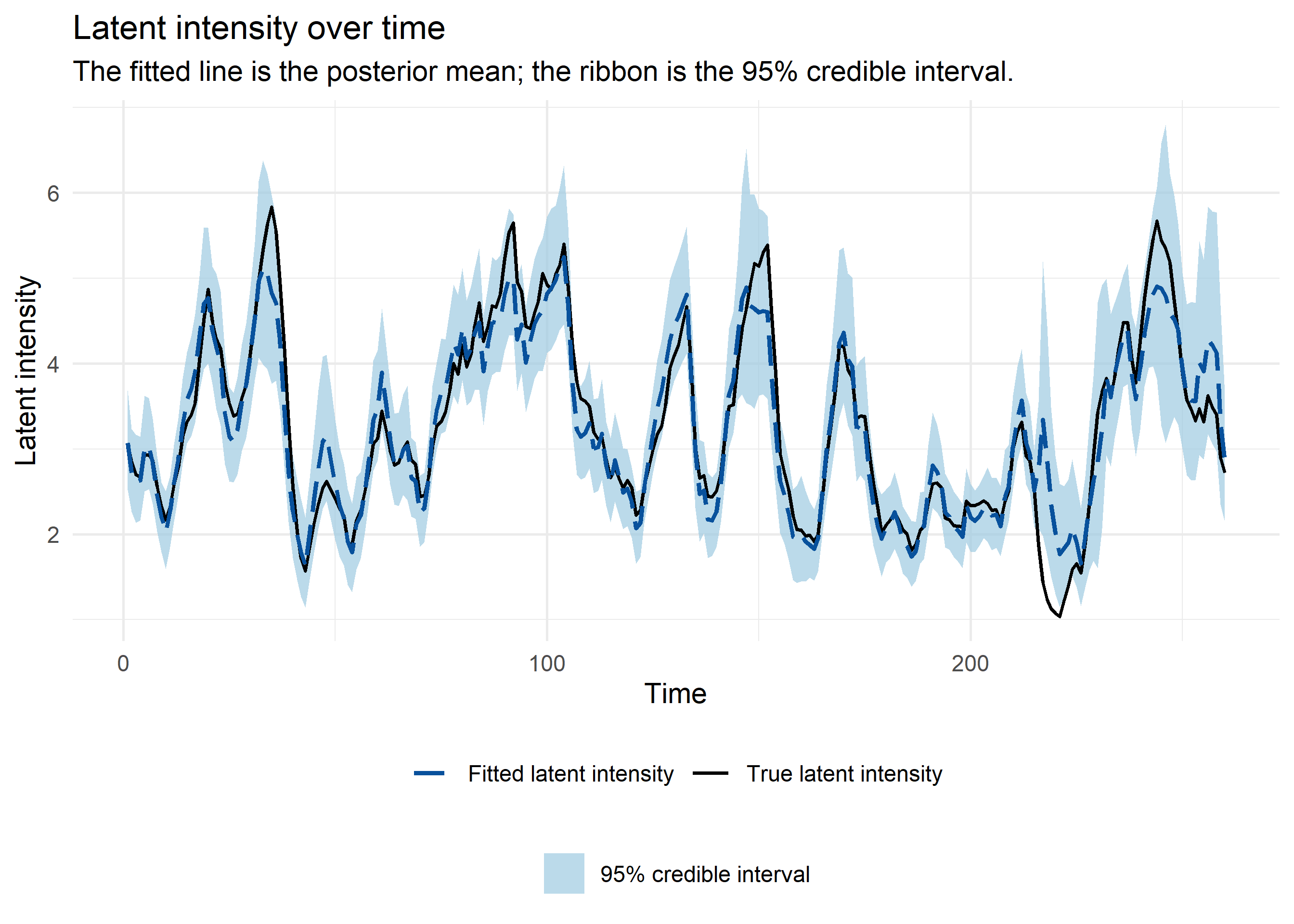
The latent-intensity plot is a useful simulation check, but it is not a posterior predictive check. The model was fitted to one noisy Poisson count at each time point, not to the black latent-intensity curve. Local departures between the fitted line and the simulated truth can therefore occur even when the DLNM structure is appropriate. The posterior predictive check below added the Poisson observation layer back in.

Posterior predictive check

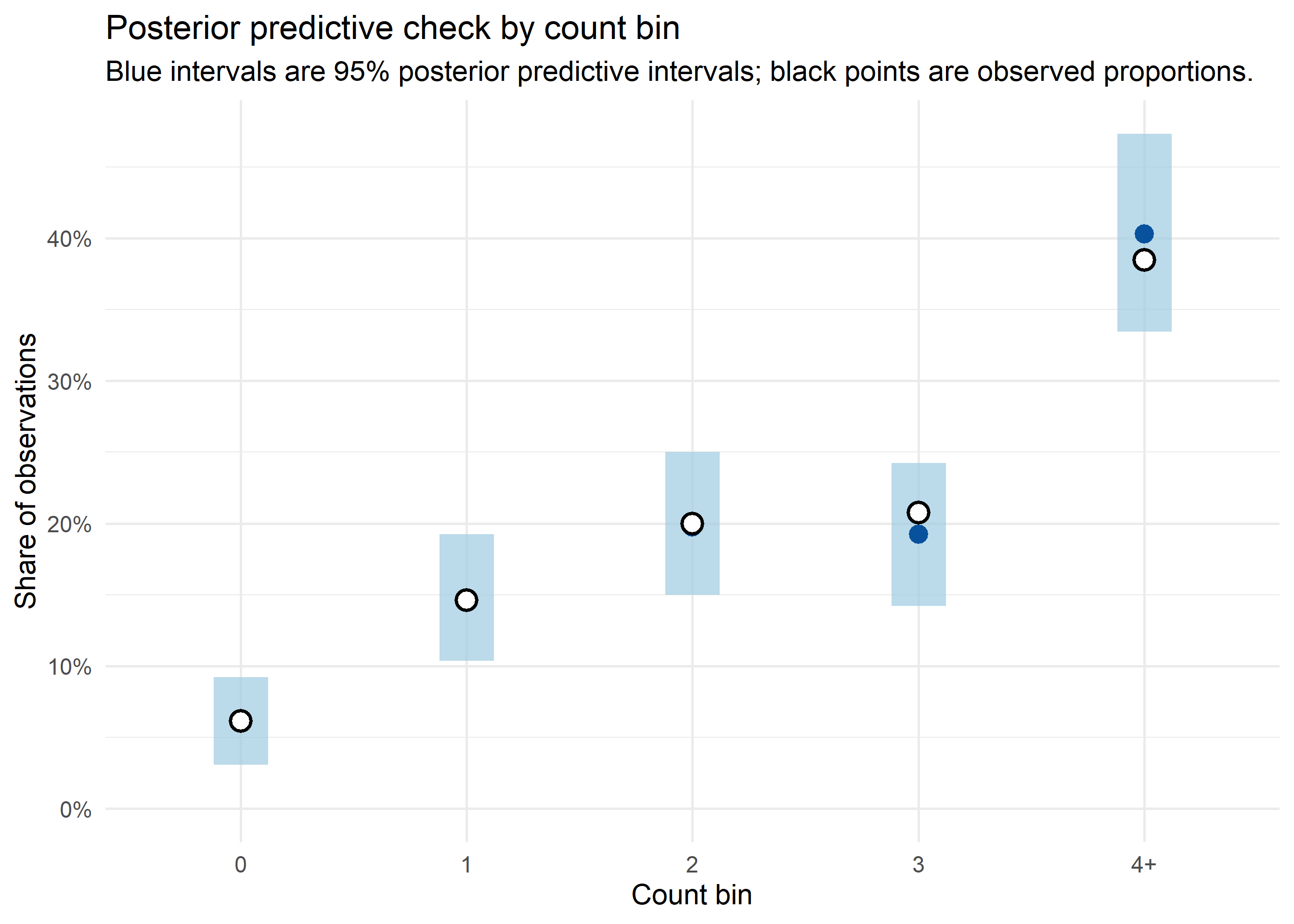
For the posterior predictive check, I added the observation noise back in. The predict() call below sampled the latent mean \(\mu_t = \exp(\alpha + A_t\theta)\), rpois() drew replicated counts from the Poisson observation model, and the result was reduced to count-bin proportions. This checked whether the fitted model reproduced the discrete distribution of the observed response, rather than only the latent mean.

count_bins <- c("0", "1", "2", "3", "4+")

bin_counts <- function(z) {
  cut(
    z,
    breaks = c(-Inf, 0, 1, 2, 3, Inf),
    labels = count_bins,
    right = TRUE
  )
}

observed_prop <- as.vector(prop.table(table(
  factor(bin_counts(y), levels = count_bins)
)))

posterior_predictive_bins <- predict(
  fit_dlnm,
  formula = ~ {
    y_rep <- rpois(
      n = length(dlnm),
      lambda = exp(Intercept + dlnm)
    )

    y_rep_prop <- as.vector(prop.table(table(
      factor(bin_counts(y_rep), levels = count_bins)
    )))

    data.frame(prop = y_rep_prop)
  },
  n.samples = 1000,
  seed = 20260426
)

posterior_predictive_bins$bin <- factor(count_bins, levels = count_bins)
posterior_predictive_bins$observed <- observed_prop

ggplot(posterior_predictive_bins, aes(x = bin)) +
  geom_linerange(
    aes(ymin = q0.025, ymax = q0.975),
    fill = "#9ecae1",
    colour = "#9ecae1",
    linewidth = 10,
    alpha = 0.7
  ) +
  geom_point(aes(y = mean), colour = "#08519c", size = 3) +
  geom_point(
    aes(y = observed),
    shape = 21,
    fill = "white",
    colour = "black",
    stroke = 1,
    size = 3.2
  ) +
  scale_y_continuous(
    labels = function(z) paste0(round(100 * z), "%"),
    limits = c(0, NA)
  ) +
  labs(
    x = "Count bin",
    y = "Share of observations",
    title = "Posterior predictive check by count bin",
    subtitle = "Blue intervals are 95% posterior predictive intervals; black points are observed proportions."
  )

Reconstructing the surface

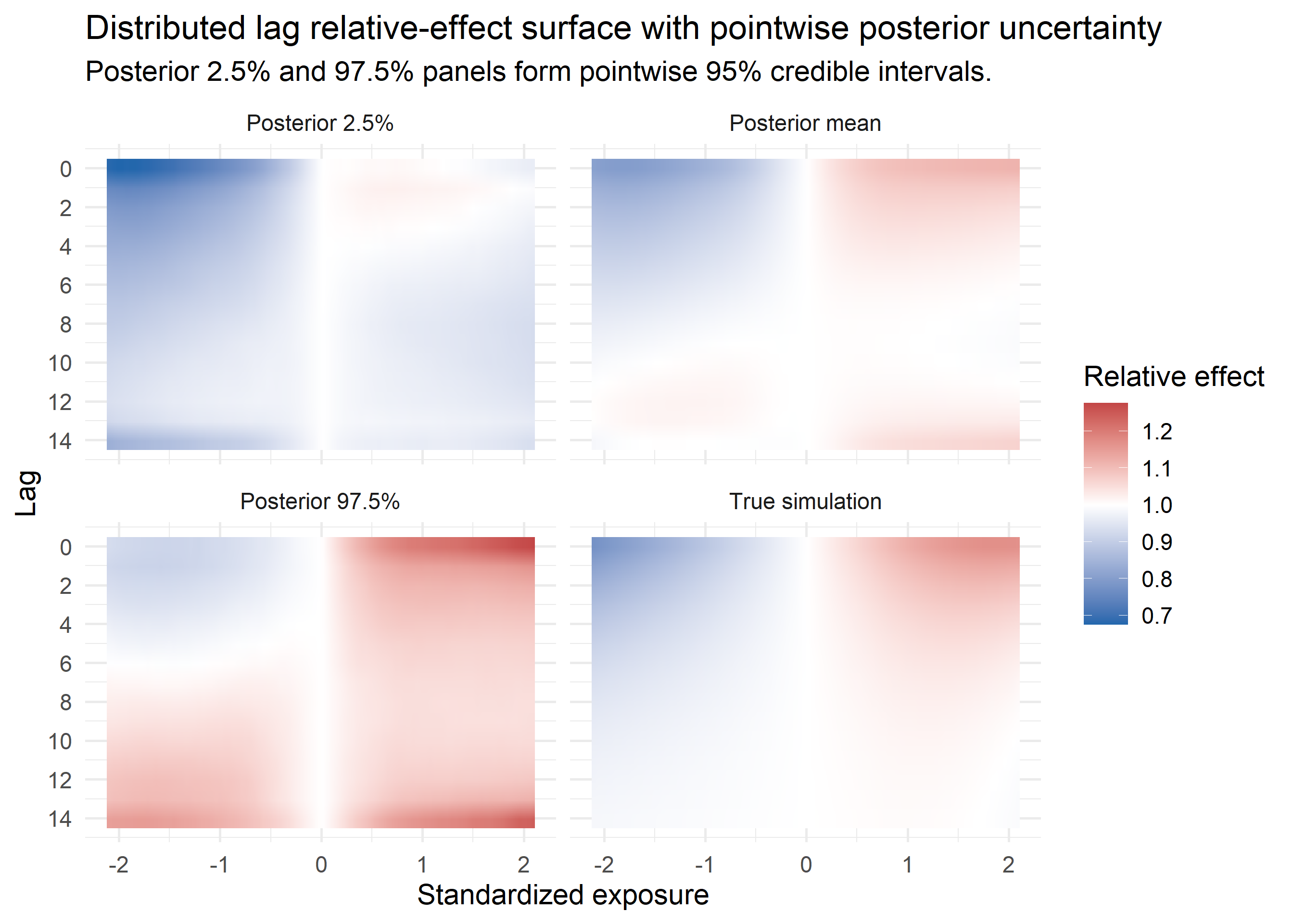
To reconstruct the fitted surface, I evaluated the DLNM component on a regular exposure-lag grid. I subtracted the fitted effect at the reference exposure \(x = 0\) on the linear-predictor scale, then exponentiated the result. The plotted surface was therefore a lag-specific relative effect.

exposure_grid <- seq(
  quantile(as.vector(x_history), 0.02),
  quantile(as.vector(x_history), 0.98),
  length.out = 100
)

reference_exposure <- 0

exposure_basis_grid <- do.call(
  onebasis,
  c(list(x = exposure_grid), attr(cross_basis, "argvar"))
)
exposure_basis_reference <- do.call(
  onebasis,
  c(list(x = reference_exposure), attr(cross_basis, "argvar"))
)
lag_basis_grid <- do.call(
  onebasis,
  c(list(x = lag_grid), attr(cross_basis, "arglag"))
)

exposure_basis_diff <- (
  exposure_basis_grid -
    matrix(
      exposure_basis_reference,
      nrow = nrow(exposure_basis_grid),
      ncol = k_exposure,
      byrow = TRUE
    )
)

surface_design <- do.call(
  rbind,
  lapply(seq_len(nrow(lag_basis_grid)), function(j) {
    do.call(
      rbind,
      lapply(seq_len(nrow(exposure_basis_diff)), function(i) {
        kronecker(exposure_basis_diff[i, ], lag_basis_grid[j, ])
      })
    )
  })
)

surface_posterior <- predict(
  fit_dlnm,
  newdata = list(A_cross = Matrix(surface_design, sparse = TRUE)),
  formula = ~ data.frame(effect = exp(dlnm)),
  n.samples = 1000,
  seed = 20260428
)

log_effect_true <- outer(
  exposure_grid,
  lag_grid,
  Vectorize(function(z, lag) {
    true_lag_effect(z, lag) - true_lag_effect(reference_exposure, lag)
  })
)

effect_true <- exp(log_effect_true)

surface_grid <- data.frame(
  exposure = rep(exposure_grid, times = length(lag_grid)),
  lag = rep(lag_grid, each = length(exposure_grid))
)

surface_df <- rbind(
  data.frame(
    surface_grid,
    effect = surface_posterior$q0.025,
    surface = "Posterior 2.5%"
  ),
  data.frame(
    surface_grid,
    effect = surface_posterior$mean,
    surface = "Posterior mean"
  ),
  data.frame(
    surface_grid,
    effect = surface_posterior$q0.975,
    surface = "Posterior 97.5%"
  ),
  data.frame(
    surface_grid,
    effect = as.vector(effect_true),
    surface = "True simulation"
  )
)

surface_df$surface <- factor(
  surface_df$surface,
  levels = c("Posterior 2.5%", "Posterior mean", "Posterior 97.5%", "True simulation")
)

ggplot(surface_df, aes(x = exposure, y = lag, fill = effect)) +
  geom_raster(interpolate = TRUE) +
  facet_wrap(~surface, ncol = 2) +
  scale_y_reverse(breaks = seq(0, max_lag, by = 2)) +
  scale_fill_gradient2(
    low = "#2166ac",
    mid = "white",
    high = "#b2182b",
    midpoint = 1
  ) +
  labs(
    x = "Standardized exposure",
    y = "Lag",
    fill = "Relative effect",
    title = "Distributed lag relative-effect surface with pointwise posterior uncertainty",
    subtitle = "Posterior 2.5% and 97.5% panels form pointwise 95% credible intervals."
  )

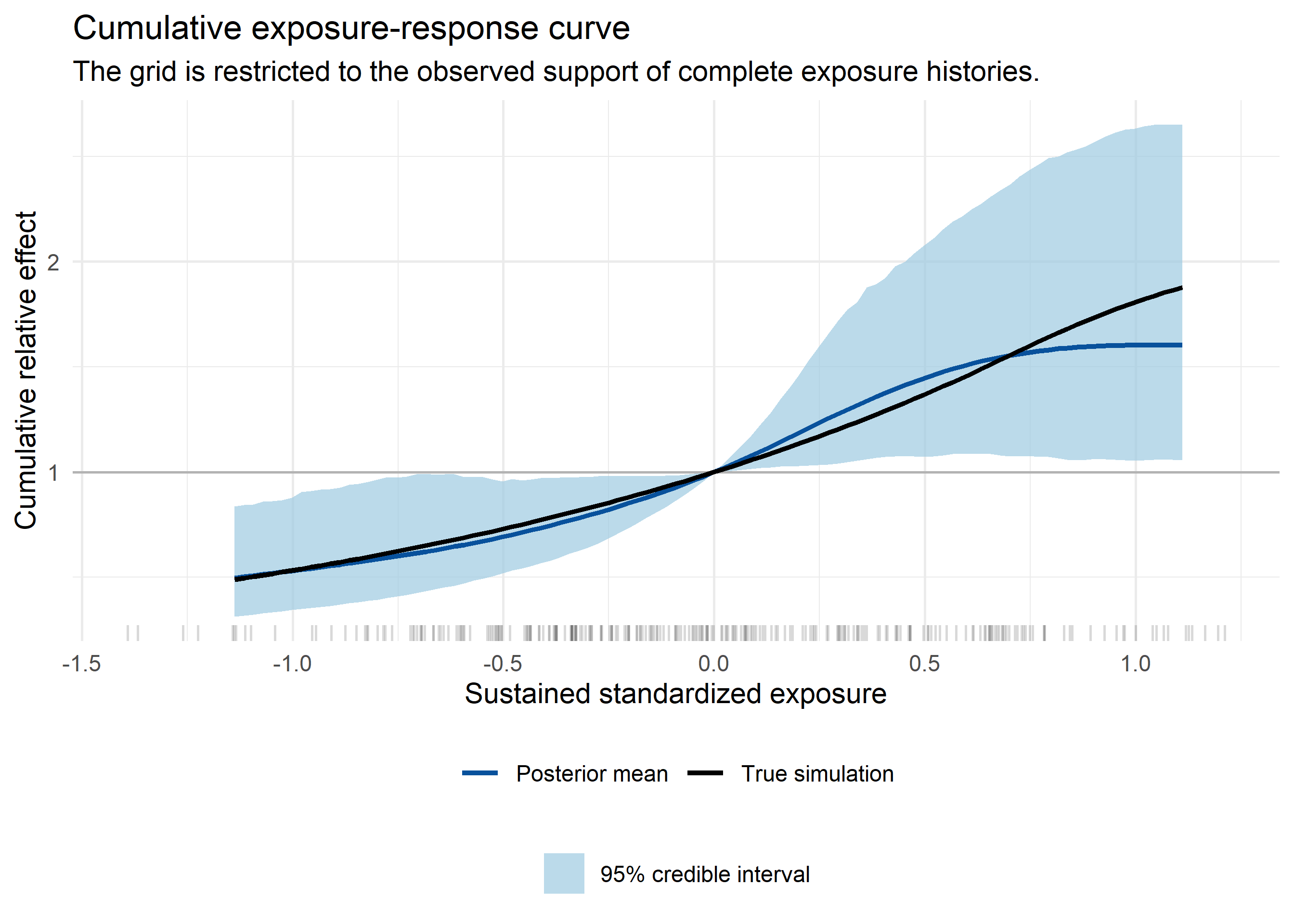
A cumulative exposure-response curve was obtained by summing the lag-specific effects over \(\ell = 0,\ldots,L\) on the linear-predictor scale and then exponentiating. In this example, it answered a concrete question: what total relative effect would we get if the same standardized exposure value were sustained throughout the whole lag window? A negative sustained exposure meant a below-average standardized exposure held constant over all lags.

For this curve, I used a more conservative exposure grid than in the surface plot. The surface plot used the marginal range of all lagged exposures, but a sustained exposure is a full exposure history. Asking for all lags to be held at a marginal tail value would extrapolate beyond the histories that were actually observed. I therefore based the cumulative grid on the central range of the row-wise mean exposure history.

cumulative_exposure_grid <- seq(
  quantile(rowMeans(x_history), 0.02),
  quantile(rowMeans(x_history), 0.98),
  length.out = length(exposure_grid)
)

cumulative_exposure_basis <- do.call(
  onebasis,
  c(list(x = cumulative_exposure_grid), attr(cross_basis, "argvar"))
)

cumulative_exposure_basis_diff <- (
  cumulative_exposure_basis -
    matrix(
      exposure_basis_reference,
      nrow = nrow(cumulative_exposure_basis),
      ncol = k_exposure,
      byrow = TRUE
    )
)

cumulative_surface_design <- do.call(
  rbind,
  lapply(seq_len(nrow(lag_basis_grid)), function(j) {
    do.call(
      rbind,
      lapply(seq_len(nrow(cumulative_exposure_basis_diff)), function(i) {
        kronecker(cumulative_exposure_basis_diff[i, ], lag_basis_grid[j, ])
      })
    )
  })
)

cumulative_surface_samples <- generate(
  fit_dlnm,
  newdata = list(A_cross = Matrix(cumulative_surface_design, sparse = TRUE)),
  formula = ~ data.frame(log_effect = dlnm),
  n.samples = 1000,
  seed = 20260429
)

cumulative_log_effect_true <- outer(
  cumulative_exposure_grid,
  lag_grid,
  Vectorize(function(z, lag) {
    true_lag_effect(z, lag) - true_lag_effect(reference_exposure, lag)
  })
)

cumulative_sample_matrix <- vapply(
  cumulative_surface_samples,
  function(sample) {
    exp(
      rowSums(matrix(
        sample$log_effect,
        nrow = length(cumulative_exposure_grid),
        ncol = length(lag_grid)
      ))
    )
  },
  numeric(length(cumulative_exposure_grid))
)

cumulative_summary <- data.frame(
  exposure = cumulative_exposure_grid,
  lower = apply(cumulative_sample_matrix, 1, quantile, probs = 0.025),
  effect = rowMeans(cumulative_sample_matrix),
  upper = apply(cumulative_sample_matrix, 1, quantile, probs = 0.975),
  curve = "Posterior mean"
)

cumulative_df <- rbind(
  cumulative_summary,
  data.frame(
    exposure = cumulative_exposure_grid,
    lower = NA_real_,
    effect = exp(rowSums(cumulative_log_effect_true)),
    upper = NA_real_,
    curve = "True simulation"
  )
)

ggplot(cumulative_df, aes(x = exposure, y = effect, colour = curve)) +
  geom_hline(yintercept = 1, colour = "grey70") +
  geom_ribbon(
    data = subset(cumulative_df, curve == "Posterior mean"),
    aes(x = exposure, ymin = lower, ymax = upper, fill = "95% credible interval"),
    inherit.aes = FALSE,
    alpha = 0.7
  ) +
  geom_line(linewidth = 0.9) +
  geom_rug(
    data = data.frame(exposure = rowMeans(x_history)),
    aes(x = exposure),
    inherit.aes = FALSE,
    sides = "b",
    alpha = 0.15
  ) +
  scale_colour_manual(values = c("Posterior mean" = "#08519c", "True simulation" = "black")) +
  scale_fill_manual(values = c("95% credible interval" = "#9ecae1")) +
  guides(
    colour = guide_legend(order = 1),
    fill = guide_legend(order = 2)
  ) +
  labs(
    x = "Sustained standardized exposure",
    y = "Cumulative relative effect",
    colour = NULL,
    fill = NULL,
    title = "Cumulative exposure-response curve",
    subtitle = "The grid is restricted to the observed support of complete exposure histories."
  ) +
  theme(
    legend.position = "bottom",
    legend.box = "vertical"
  )

Notes

This construction was deliberately explicit. In a real analysis, I would add the usual time-series structure around the DLNM term: seasonal terms, long-term trend, calendar effects, overdispersion if the Poisson variance is too small, and possibly autocorrelated residual structure. The cross-basis term is only one part of the linear predictor.

The main technical point was simple: once the exposure histories had been converted into a cross-basis matrix, the DLNM became a linear model component. From there, inlabru could fit it as a latent Gaussian component, with the prior structure controlled through the list of precision matrices passed to generic3.

An alternative to generic3 is generic0, which uses a single precision parameter for the whole combined penalty matrix. In the notation used above, this corresponds to replacing the two-precision structure

\[ \tau_\ell R_\ell + \tau_x R_x \]

with the simpler one-precision structure

\[ \tau (R_\ell + R_x). \]

In settings with substantial uncertainty, as in this small simulated example, that simpler latent effect can be preferable because it reduces the number of smoothing hyperparameters that must be learned from the data. I used generic3 here because it is more general and makes the exposure-direction and lag-direction regularisation explicit.